User Manual
Introduction
The aim of creating the Ship Simulation Workbench is to provide the framework for the performance estimation of a ship sailing on different routes and under realistic service conditions, i.e., with waves, wind and limited water depth. Interaction between the engine and propeller is included while simulating voyages, so the estimate of the ship performance consists of, power, energy consumption, possible delays due to weather. Ship simulation workbench provides voyage performance considering all the interactions between hull, propeller, engine and weather conditions.
Ship Simulation Workbench provides the flexibility to include user specified calm water resistance and propeller openwater curves. E.g., calm water resistance can be estimated using an empirical approach, model test data or CFD simulations. Hence, the industry or academic groups can continue using the methods of their preference and still be able to estimate the vessel performance in Ship Simulation Workbench.
For the user who are not expert in Naval Architecture, basic empirical methods have been provided which require minimal inputs. E.g. if exact propeller details are unknown, workbench can design an appropriate propeller which will be used for voyage simulations.
Ship simulation workbench can be cited as follows:
Taskar Bhushan, Andersen Poul.(2019) Ship Simulation Workbench: User Manual. Technical University of Denmark. www.SSW.mek.dtu.dk
Units
Units for different parameters in ship simulation workbench are as follows:
| Parameter | Unit |
|---|---|
| Length | m |
| Surface ares | m2 |
| Distance | nautical miles |
| Speed | m/s |
| Power | kW |
| Torque | kN.m |
| Thrust | kN |
| Resistance | kN |
| Money | USD |
Input file types
Two different formats are used in ship simulation workbench for input files. Each file needs to be in a specific format in order to be read correctly.
- Format 1: json
These file types start and end with curly brackets{}. There are double quotes "" for variable name, and variables are separated with comma. hull_prop_engine, guldhammer, holtrop, hollenbach and wind resistance files are in this format. It is necessary that these files are valid json files. It can be checked using the following link.
Check if input file is valid
- Format 2: Data in column format
In this case data are supplied as multiple columns separated by a space or a tab. Engine SFOC, calm_resistance, custom openwater curves, weather and route files are of this type. In the case of these files, it's a good idea to prepare columns in excel file and copy-paste the table into text file. In this file format, lines starting with # are ignored.
Ship details
hull_prop_engine.txt is the file that contains principal particulars about hull geometry, propeller details, propulsion factors and engine particulars. Parameters have been grouped in four sections- Hull, Propeller, Propulsion and Engine.
hull_prop_engine.txt for KVLCC2 hull_prop_engine.txt for KCSHull
L: ship length (Length between perpendiculars)
B: breadth
T: draft
Cb: block coefficient
V: design speed
S: wetted surface area
Cm: midship section coeff. It is utilized only by Holtrop and by Guldhammer and Harvald methods to calculate calm water resistance and by Lackenby method for the calculation of ship speed or resistance in shallow water. It can be left empty like [] if these methods are not being used.
Cwp: waterplane area coeff. It is utilized only by Holtrop method to calculate calm water resistance and by Raven method for the calculation of ship speed or resistance in shallow water. It can be left empty like [] if these methods are not being used.
ship_type: type of ship (’bulker’, ’tanker’, ’container’ or ’roro’). This is used for the calculation of propeller diameter if it is not specified (left empty like []).
ks: roughness of hull surface in micrometers.
Propeller
Z: no. of propeller blades
Dia: propeller diameter. It can be left empty like [] and the program will automatically chose it if ship type is ’bulker’, ’tanker’, ’container’ or ’roro’.
PoD: pitch/diameter ratio.
EAR: expanded area ratio. It will be approximated if ’design appropriate propeller’ option is chosen in Propeller openwater curves. Otherwise specified value will be used.
h: submergence of propeller center. It is required for the calculation of EAR only if ’design appropriate propeller’ option is chosen in Propeller openwater curves.
design_rpm: Design speed of the propeller. It is automatically calculated only if ’design appropriate propeller’ option is chosen.
Propulsion
w: wake fraction. It is approximated using L, B, Cb and propeller diameter if left blank []
t: thrust deduction. It is approximated using L, B, Cb and propeller diameter if left blank []
no_of_propellers: number of propellers. All propellers are assumed identical, it is also assumed that the wake fraction is identical for all the propellers.
relative_rotative: relative rotative efficiency. It is assumed equal to one if left empty [].
trans_effi: transmission efficiency. It is assumed equal to one if left empty [].
Engine
This section is required only when 'Consider engine limits' box is checked.
MCR_P: power at MCR. Used to calculate engine load diagram only when 'Consider engine limits' is checked.
MCR_rpm: engine speed at MCR point. Used to calculate engine load diagram only when 'Consider engine limits' is checked. Max rpm is assumed 5% greater than MCR_rpm.
gear_ratio: gear ratio.
Simulation Methods
In this section, provides an overview of different methods available in the workbench. Some of the methods require additional inputs which should be provided in certain format.
Calm water resistance
Following methods are available for the calculation of calm water resistance. An additional input file specific to each method is required for the calculation of calm water resistance. Additional inputs and the format of input file are as follows.-
Guldhammer and Harvald
Guldhammer and Harvald's method [1] is available along with the corrections provided by Kristensen [2]. Input file with following variables should be provided. The input file should be in format 1 as shown in example files. The explanation of variables is as follows.
guldhammer.txt for KVLCC2 guldhammer.txt for KCSLpp: length between perpendiculars.
Laft: distance from the aft limit of the displacement to AP. This value may be negative if aft limit is forward of AP.
Lfore: distance from FP to the fore limit of the displacement. This value may be negative if fore limit is aft of FP.
LCB0: distance of longitudinal center of buoyancy from the midship section (Lpp/2) positive aft.
Ff: shape of fore body. It varies between -3 and 3. 3 for extreme U-shape, 0 for N shape and -3 for V-shape.
Fa: shape of aft body. It varies between -3 and 3. 3 for extreme U-shape, 0 for N shape and -3 for V-shape.
Capp: total correction for appendages must be specified as a percentage of residuary resistance coefficient.
Rudder: no correction for normal rudders. The standard form has a single rudder.
Bilge keels: no correction.
Bossings: for full ship forms 3-5 percent.
shaft brackets and shafts: For fine ship forms 5-8 percent.
These corrections should be significantly smaller than the residuary resistance coefficient.
deltaS: total wetted surface of appendages.
bulb_area_ratio: the ratio of the sectional area at the fore perpendicular to the midship section area.
new_correction: If Guldhammer's method updated by Kristensen should be used. 1 for using the corrections, 0 for using the original method.
-
Holtrop
Variables to be provided in the input file for this method are listed below. The input file should be in format 1. Some of the variables are optional which means if the value is not provided then those are estimated using the regression formulae provided by Holtrop. Empty brackets [] must be used if optional parameters are to be left unspecified.
holtrop.txt for KVLCC2Lwl: length of waterline
A_T: immersed area of transom at rest
A_BT: transverse area of bulbous bow
h_B: centre of area of A_BT above the keel
i_E: half angle of entrance of the waterline at the fore end (optional)
T_F: draft forward.
k: form factor. (C_stern is required if k is not provided)
Cwp: waterplane area coefficient. (optional)
LCB: LCB forward of 0.5L as a percentage of L.
C_stern: stern shape parameter which is used to calculate k if it is not provided. Values can be taken from the table below based on the stern form of the ship. Not required if k is available.
C_stern parameter Afterbody form C_stern Pram with gondola -25 V-shaped sections -10 Normal section shape 0 U-shaped sections with Hogner stern 10 L_R: length of run (optional)
k2: list of appendage form factors. e.g. [k21, k22, k23] corresponding to appendages a1, a2, a3. k2 can be obtained from the values suggested by holtrop provided in the table below.
Appendage form factors 1+k2 Appendage type (1+k2) Rudder behind skeg 1.5–2.0 Rudder behind stern 1.3–1.5 Twin-screw balanced rudders 2.8 Shaft brackets 3.0 Skeg 1.5–2.0 Strut bossings 3.0 Hull bossings 2.0 Shafts 2.0–4.0 Stabiliser fins 2.8 Dome 2.7 Bilge keels 1.4 S_app: list of wetted area of appendage(s) to be specified in the same order of appendage form factor (k2). e.g. [s1, s2, s3] corresponding to appendages a1, a2, a3
d_T: diameter of bow thruster if the ship has bow thruster.
C_BTO: lies in the range of 0.003 to 0.012. When the thruster lies in the cylindrical part of the bulbous bow, C_BTO tends to 0.003.
-
Hollenbach
The list of variables to be included in the input file is as follows.
hollenbach.txt for KVLCC2 hollenbach.txt for KCSLwl: length of waterline.
Los: length of submerged ship. It is defined as:
for the design draught, length between the aft end of the design waterline and the forward most point of the ship below the design waterline, for example, the fore end of a bulbous bow.
for the ballast draught, length between the aft end and the forward end of the hull at the ballast waterline, for example, the fore end of a bulbous bow would be taken into account but a rudder is not taken into account.
Nrudd: Number of rudders (1 or 2)
Nbrac: Number of brackets (0 to 2)
Nboss: Number of bossings (0 to 2)
Nthr: Number of side thrusters (0 to 4)
-
Custom resistance curve
custom_calm_resistance.txt for KVLCC2 custom_calm_resistance.txt for KCSUser specified inputs can be provided for the calculation of calm water resistance. Data should be in the form of two columns. First column should be a list of ship speeds in m/s in increasing order, and second one should be calm water resistance in kN at corresponding ship speed. Resistance should be provided at least at four different speeds. Resistance at intermediate speeds is calculated using the cubic spline interpolation.
Added resistance due to waves
Two methods are available for the calculation of added resistance due to waves. Added resistance RAO are calculated using these methods. Bretschneider spectrum is used for the calculation of added resistance in irregular waves based on significant waveheight and peak period of waves.
DTU method: This method is based on strip theory, Faltinsen's method for short waves and WAMIT calculations for zero forward speed cases. The DTU method can compute the added resistance for wave headings from head sea to beam sea. Added resistance is considered zero for stern quartering and following waves. Further details and validations can be found in [3]. This method works for froude numbers less than 0.25. Added resistance RAOs using this method can be tried here.
STA-wave2: Wave heading is not taken into account in this method. Waves coming from ∓45° off bow (which means 135° to 180° wave heading) are considered head waves. More details about this method can be found here [4].
Shallow water resistance
Shallow water resistance can be calculated using the method given by Lackenby [5] or Raven [6]. No additional inputs are required for the calculation. Shallow water resistance is calculated only when user specified weather and route are used. The field 'depth' should be specified in the weather and route file for shallow water resistance to be computed.
Lackenby: This method is applicable for depth froude number between 0.6 and 0.7. and Am/H2 between 0.111 and 0.25. Where Am is midship section area and H is the water depth.
Raven: This method is applicable for depth froude number less than 0.65 and draft to water depth ratio less than 0.5.
Propeller openwater curves
Three options are available for obtaining propeller openwater curves.-
Calculate using given parameter
Openwater curves are calculated using the principle particulars of propeller provided in hull_prop_engine.txt. It is assumed to be a B-series propeller. -
Design appropriate propeller
In this case, B-series propeller is designed to produce required thrust at the design speed of ship. Required thrust is calculated based on calm water resistance at the design speed and the value of thrust deduction provided in hull_prop_engine.txt. Propeller diameter is used as an input. Expanded area ratio is also used if provided. Otherwise it is estimated using Keller's criteria. Propeller design is optimized for maximum efficiency. If propeller diameter is not specified, then it will be calculated based on empirical formulae based on ship_type specified in hull_prop_engine.txt. -
User specified
Text file with three columns J(first column), KT(second column) and KQ(third column) should be provided for custom openwater curves. KT and KQ should be provided at least at four different values of J. Check example file for the correct format. Openwater curves are interpolated using cubic spline to calculate KT and KQ at intermediate values of J.
custom_openwater.txt for KVLCC2 custom_openwater.txt for KCS
Wind resistance
Additional inputs are required for the calculation of wind resistance using the method suggested by ITTC [4]. Extra parameters required are as follows.
wind_resistance.txt for KVLCC2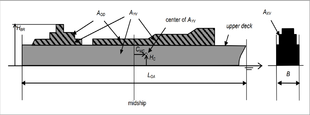
LOA: length overall.
A_OD: lateral projected area of superstructures etc. on deck.
A_XV: area of maximum transverse section exposed to the winds.
A_YV: projected lateral area above the waterline.
C_MC: horizontal distance from midship section to centre of lateral projected area A_YV. Positive forward.
h_BR: height of top of superstructure (bridge etc.)
h_C: height from waterline to centre of lateral projected area A_YV.
Weather and Route
- Monthly averaged weather conditions
Weather data averaged over each month in year 2010 are included as an example. The data are taken from the Climate Data Store of Coperniucus. Wind and wave data with global coverage are available. The data consist of significant waveheight, peak period, wave direction, wind speed and wind direction.
Route file needs to be provided which in this case should contain a list of latittudes and longitudes at multiple points along the route. It is necesasry to have column headers 'lat' and 'lon' for the columns to be recognized as lattitude and longitude. Route between the given waypoints is interpolated along the great circle. Calculations are performed at multiple points along the route. It is made sure that calculation points are less than 50 nautical miles apart. Therefore, it is possible to just specify first and the last points and intermediate points will be calculated automatically. (Just make sure that there is no landmass in between!)
Example route file from Los Angeles to Osaka
Example route file from Panama to Auckland
Example route file from Halifax to Bremerhaven
- User specified weather
It is possible to user user specified weather conditions instead of default monthly weather. In this case, various weather parameters will be provided by the user along the route. Both weather and route will be provided in the same file. Weather data like Hs, Tp, wave direction, wind speed and wind direction should be specified at each point along the route. In addition to the weather data, 'depth' can also be specified for the calculation of shallow water resistance. It is made sure that calculation points are less than 50 nautical miles apart. Additional waypoint will be introduced along the great circle between the waypoints that are farther than 50 nautical miles. In such a case, weather data and depth will also be interpolated at intermediate waypoint. Data should be given in the form of columns. Data in each column will be recognized based on column header. Following headers should be used for weather data.
- lat: Lattitude
- lon: Longutude
- Hs: Significant waveheight
- Tp: Peak period
- wave_dir: Wave direction in ship or global frame of reference. Check 'Frame of reference' section for the definition of direction.
- wind_V: Wind speed
- wind_dir: Wind direction in ship or global frame of reference. Check 'Frame of reference' section for the definition of direction.
Tip: It's a good idea to prepare the table in an Excel sheet with above headings. After filling all the values, the whole table can be pasted into a text file.
Frame of reference: Drop down meny should be used to specify if wave and wind directions are in ship frame of reference or global frame of reference.
- Ship frame of reference: Wind and wave directions shoule be specified with respect to ship. 180° means head waves and 0° means following waves. Simillarly for wind, 180° is head wind and 0° is tail wind. These values are directly used to calculate wind and wave resistance.
- Global frame of reference: Wind and wave directions shoule be specified in earth fixed co-ordinate system. Coming from north is 0° and coming from east is 90° both for wind and waves. These values along with ship speed and heading are used to calculate wave direction, wind direction and wind speed in ship frame of reference, which is then used to calculate wind and wave resistance.
Example file with weather and route.
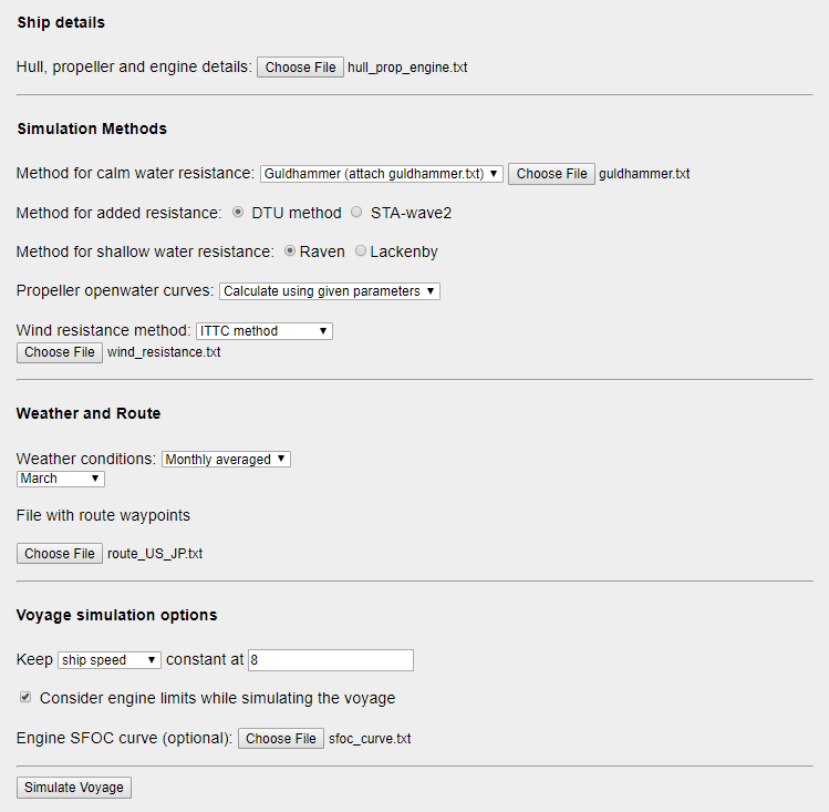
Voyage simulation options
Voyages can be simulated at constant ship speed, propeller speed or engine power. The value of speed, rpm or power to be kept constant should be specified in each case. In the case of constant ship speed, propeller rpm and engine power will be adjusted to keep the ship speed constant at the specified value.
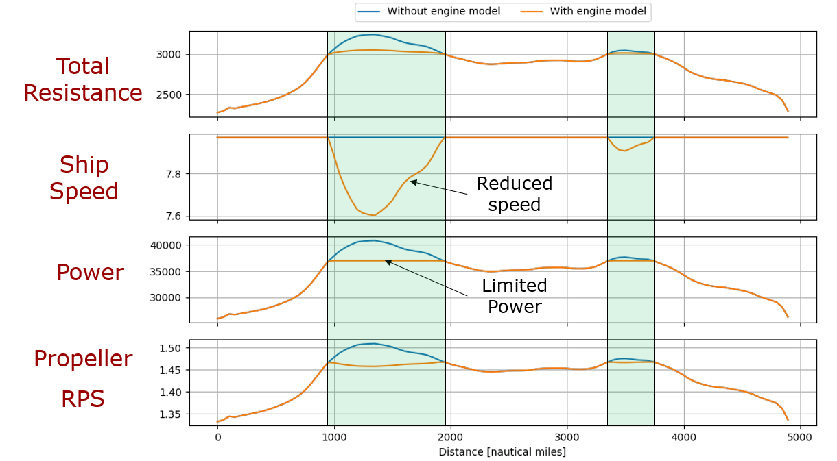
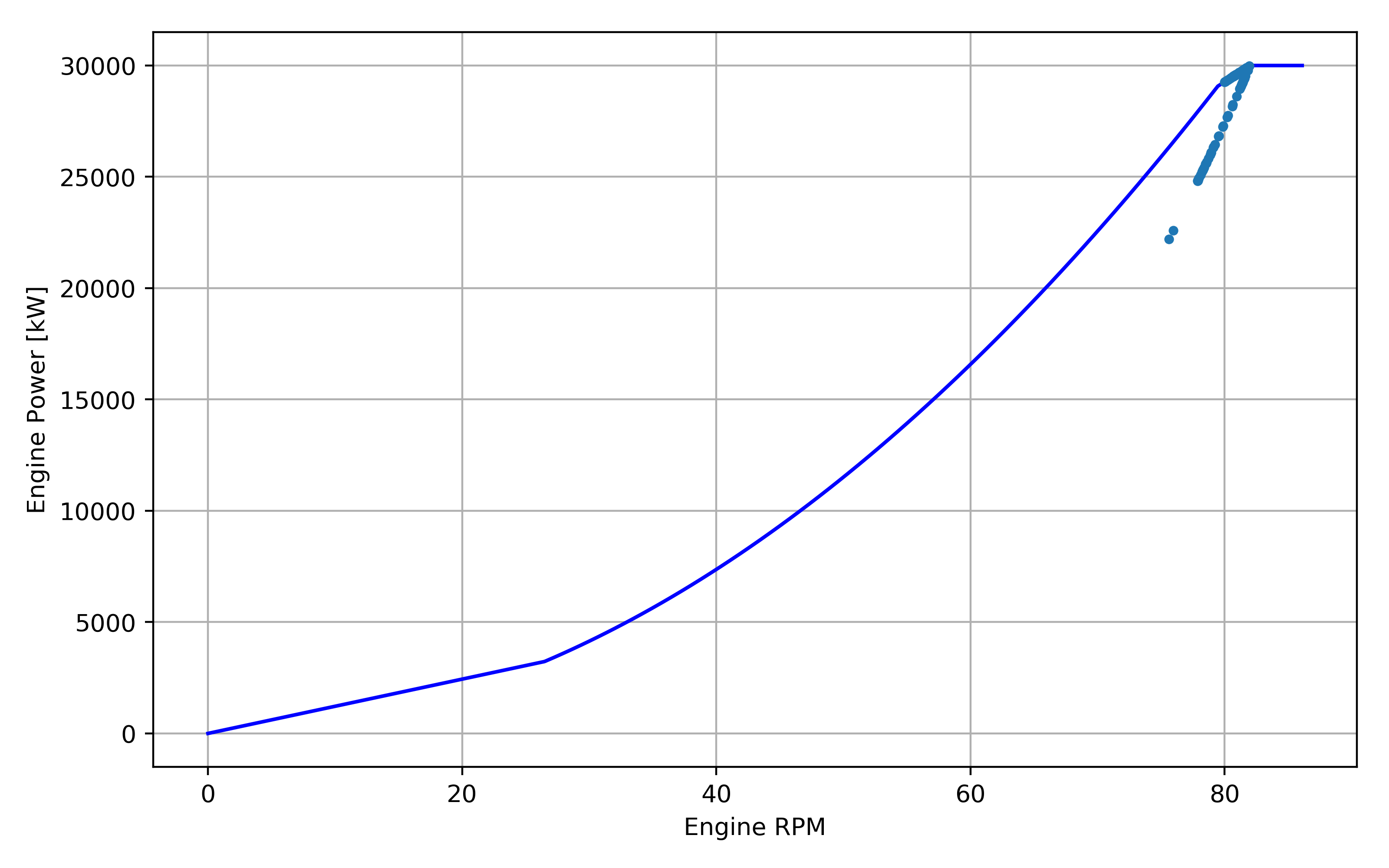
Consider engine limits: The engine load diagram will be created using MCR_P and MCR_rpm provided in hull_prop_engine file. The method suggested by MAN Energy Solutions [7] has been followed for obtaining engine load diagram. The workbench will make sure that the engine is operating withing the limits during the voyage. In the case of constant ship speed simulations, if the required power to keep ship speed constant is higher than the available power, then engine speed and ship speed will be reduced. In that case, propeller rpm and ship speed will be calculated for maximum available power. An example of this can be seen in the following figure.
Engine SFOC curve: Engine specific fuel consumption curve can only be provided when 'consider engine limits' is selected. fuel_consumption.txt should consist of two columns and at least four rows(data points). Cubic interpolation is used to calculate SFOC at intermediate values. First column listing percentage engine loads and second column should contain corresponding SFOC values in g/kWh. If the file is not provided then engine SFOC is assumed constant (160 g/kWh) for all engine loads. Engine calculation tool can be used for engine selection as well as for obtaining SFOC curve.
Example file for SFOC curve.
Simulation Results
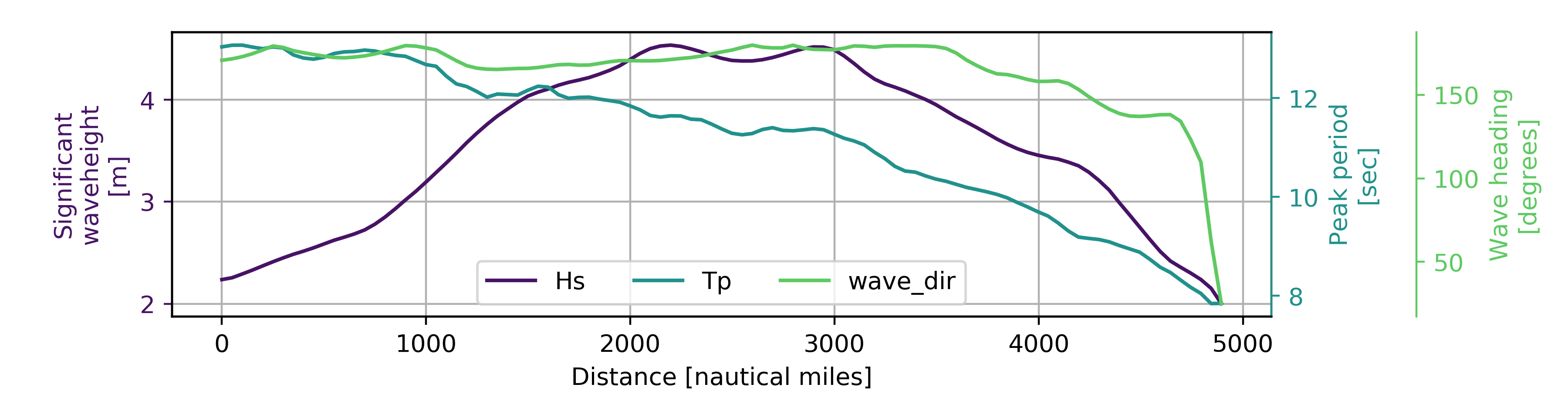
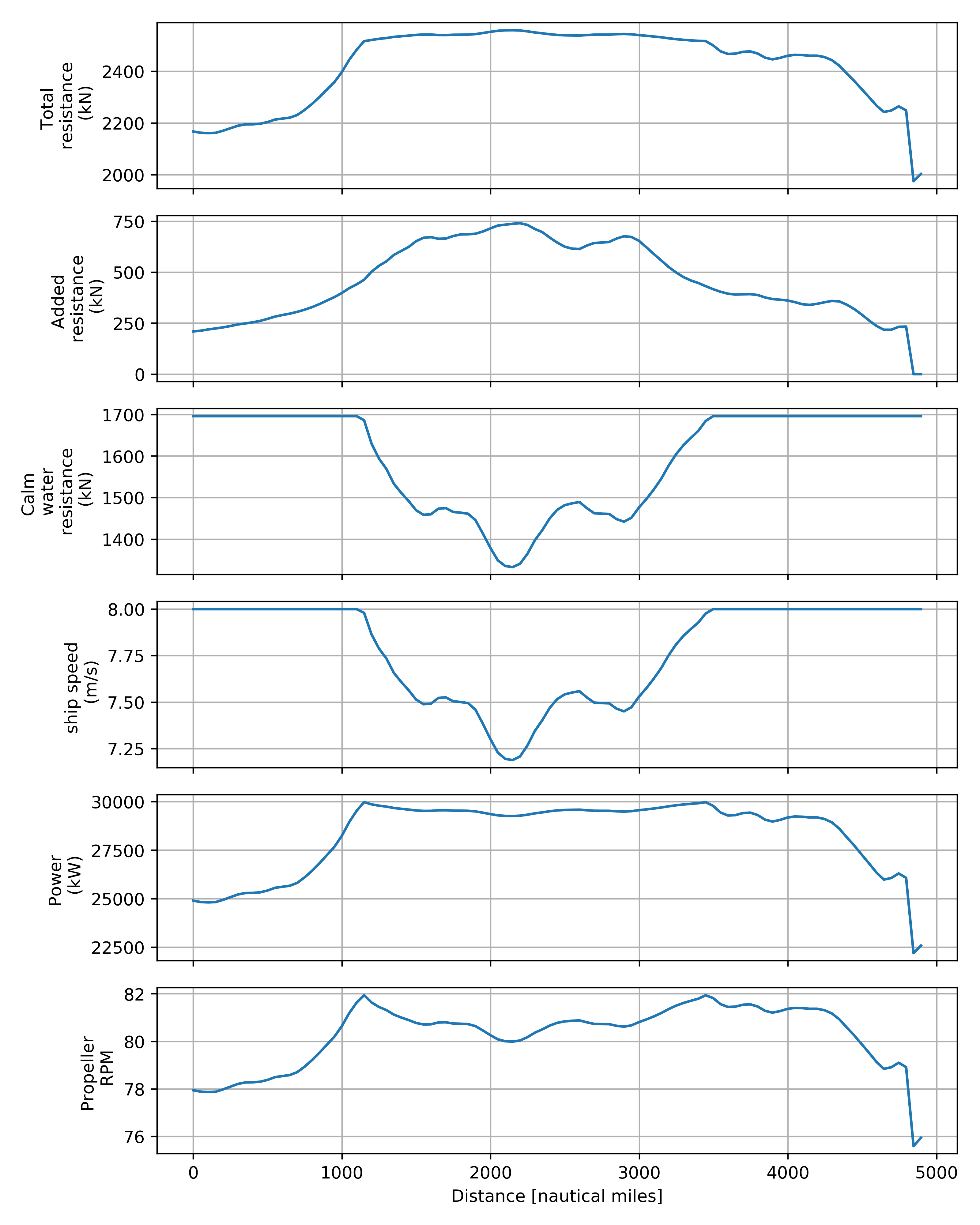
Simulation results are shown on a separate webpage in the form of multiple plots. If monthly averaged weather is used, then weather and route are plotted on the same map. In the case of user specified weather, only route is shown. Significant waveheight, peak period and wave heading are plotted along the route(180°: head waves; 0°: following waves). Simulation results like resistance, power, propeller speed and ship speed are plotted at multiple points along the route.
If the option of engine limits is selected, then RPM and power at multiple points along the route are shown along with the engine limits. If 'consider engine limits' option is not selected then only power and RPM are plotted.
It is also possible to download the entire simulation data by clicking 'Download simulation data' button. A CSV file will be downloaded. The data provide vessel performance at multiple points along the route. Variables in CSV file are as follows.
- lat: Lattitude
- lon: Longitude
- w_L: Wavelength/ship length for the wave corresponding to peak period.
- dist: Distance from start of the route to current point. This can be used to plot different quantities along the route.
- hours: Hours taken to travel from current waypoint to the next waypoint.
- tot_r: Total resistance
- shallow_r: Shallow water resistance
- wind_r: Wind resistance. This can be negative in case of tailwind.
- added_r: Added resistance in waves.
- calm_r: Calm water resistance.
- V: Ship speed.
- P: Engine power.
- n: Propeller speed (RPS).
- Hs: Significant waveheight at the location.
- Tp: Peak period at the location.
- wave_dir: Wave direction with respect to the ship. (180°: head waves; 0°: following waves)
- wind_V: Wind speed.
- wind_dir: Wind direction with respect to the ship. (180°: head wind; 0°: tail wind)
- FC_inst: Fuel consumption for a the leg of journey from current waypoint to the next one.
Typical output
Using the input files for KVLCC2 and following options chosen on user interface, typical output has been shown below.
Monthly weather and specified route on the world map. In the case of user specified weather, only route is shown as the weather data are provided only along the route.
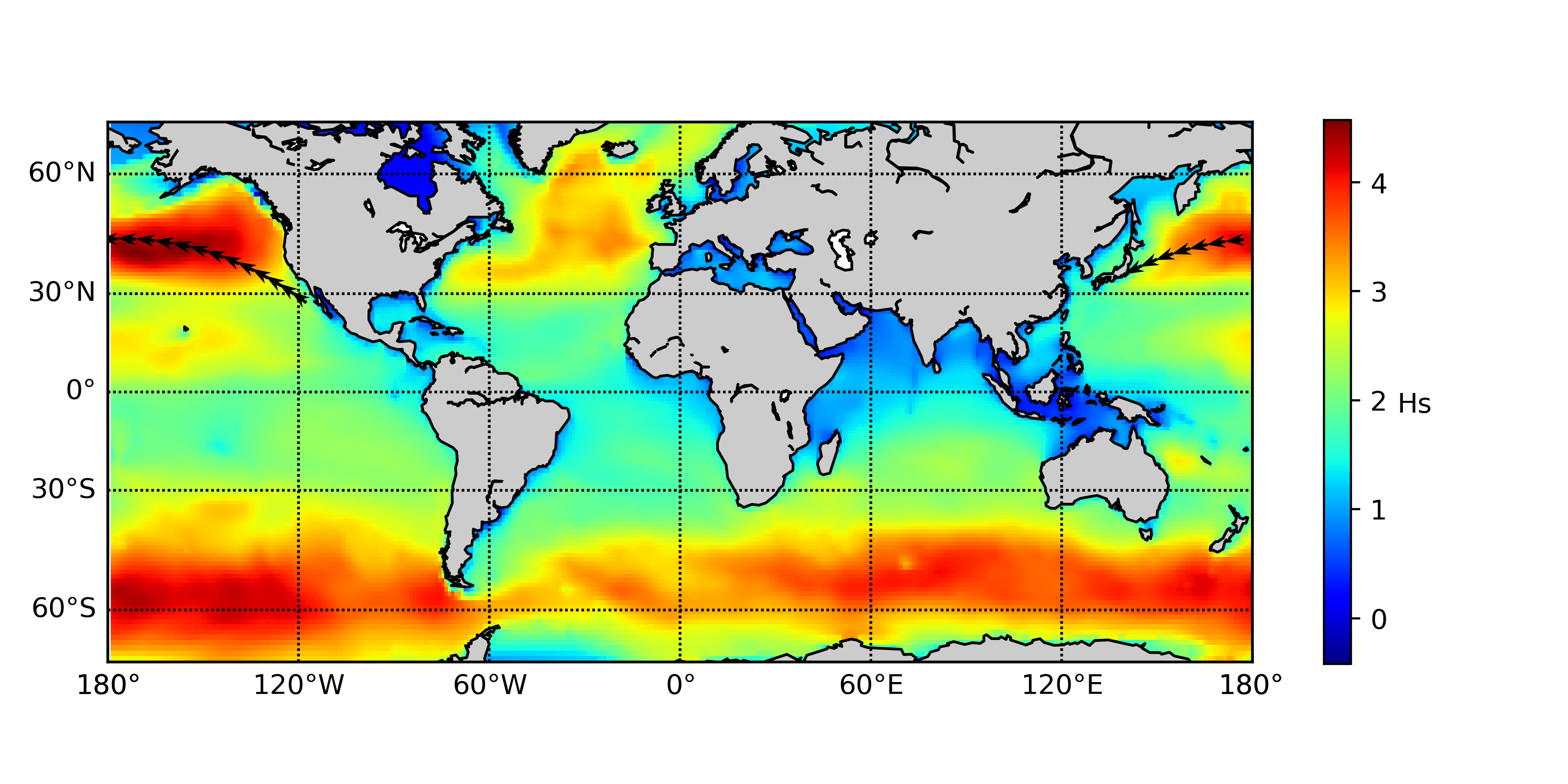
Total distance travelled = 4944 nautical miles
Voyage time = 13.6 days
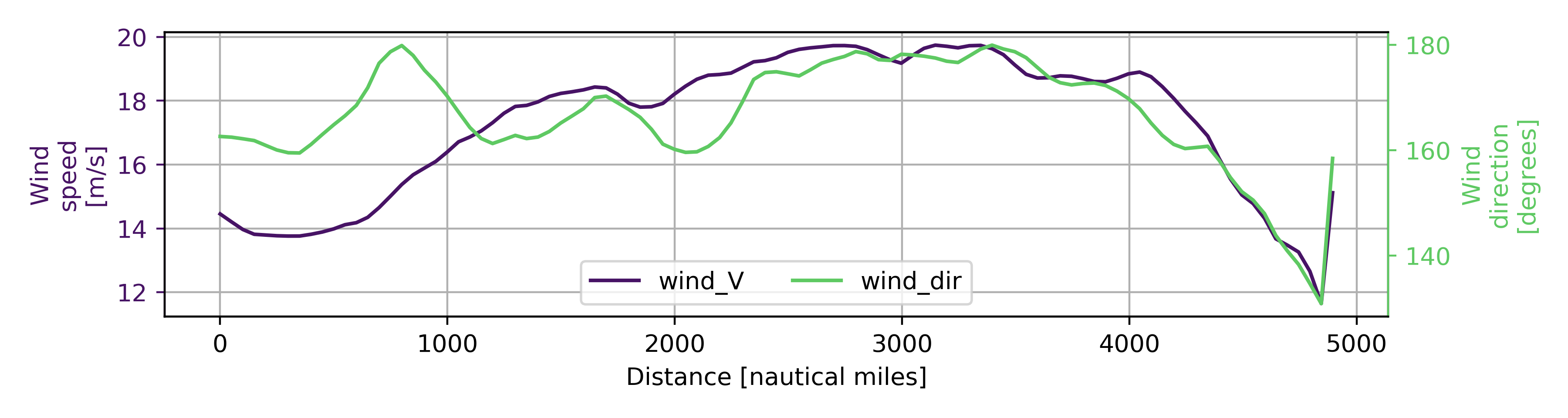
Wind and wave conditions along the route are shown. Wave direction, wind direction and wind speed are in ship frame of reference. Wind conditions are not shown when 'No wind resistance' option is selected.
Important performance indicators regarding vessel performance are shown here. More details can be found by downloading the simulation data.
Engine load diagram along with engine operating points at different locations along the route.
Total fuel consumption = 1488.0 tonnes
REFERENCES
[1] H. E. Guldhammer, S. A. Harvald, Ship Resistance - Effect of Form and Principal Dimensions, Akademisk Forlag, Copenhagen, 1974.
[2] H. O. Kristensen and M. Lützen, “Prediction of Resistance and Propulsion Power of Ships,” 2017.
[3] M. A. Martinsen, “An design tool for estimating the added wave resistance of container ships,” 2016.
[4] ITTC-Recommended Procedures and Guidelines 7.5-04-01-01.2. Speed and Power Trials, Part 2 Analysis of Speed/Power Trial Data.
[5] H. Lackenby, “The Effect of Shallow Water on Ship Speed,” Shipbuild. Mar. engine Build., vol. September, pp. 446–450, 1963.
[6] H. C. Raven, “A New Correction Procedure for Shallow Water Effects in Ship Speed Trials,” in Proceedings of PRADS 2016, 2016.
[7] MAN Energy Solutions, “Basic principles of ship propulsion,” 2018.
[8] A. F. Molland, S. R. Turnock, and D. A. Hudson, Ship Resistance and Propulsion. 2011.